TheEpicCowOfLife's Blog
Imagine reviving this blog, couldn't be me.
Project maintained by Hosted on GitHub Pages — Theme by mattgraham
Recently I had an opportunity to do some mathematical research. Basically: projection algorithms work on combinatorial problems, and I wanted to find out why. Nobody has been able to give good mathematical justification for why they work. To collate my assorted poking around, this is the start of a 3-part series on this topic.
How was I able to do mathematical research?
I had the luxury of participating in the University of Melbourne’s Mathematics and Statistics Vacation Scholarships Program. Over the course of 4 weeks, I undertook this project with my supervisor Matthew Tam.
WIP Note
I shall be stealing images from various sources with low effort screenshots, this is temporary. Hopefully.
\[\def\reals{\mathbb{R}} \newcommand{\bx}{\mathbf x} \newcommand{\bw}{\mathbf w} \newcommand{\by}{\mathbf y} \newcommand{\bz}{\mathbf z} \newcommand{\ba}{\mathbf a} \newcommand{\bv}{\mathbf v} \DeclareMathOperator{\Fix}{Fix} \newcommand{\integ}[2]{[[{#1},{#2}]]}\]Mathematical preliminaries
This particular blog post will be dedicated to establishing the mathematical background behind the algorithms investigated- without this, the following articles probably won’t make any sense. With that said, let’s get on with it!
Feasibility problems
We will be trying to solve a fairly specific type of problem: Suppose we had an Euclidean space \(E\) (loosely speaking, it’s another name for \(\reals^n\)), and \(n\) constraint sets \(C_1, C_2, \dots, C_n \subseteq E\). A feasibility problem asks to find an \(x \in E\) such that
\[x \in C_1 \cap C_2 \cap \dots \cap C_n\]or to determine that \(C_1 \cap C_2 \cap \dots \cap C_n = \varnothing\)
If you’re fairly uncreative, this could mean we’re just looking at problems where we’re literally trying to find the intersection of sets in \(\reals^n\). However, with more creativity, we can formulate more familliar problems like Sudoku, N-Queens, 3-SAT, Graph Coloring and Protein Folding. Heuristically, All that is required is for the problem to ask roughly “Can you find an x such that it satisfies all these conditions”?
Convexity
A lot of the theorems quoted later will involve convexity. Here is the definition for your pleasure.
A set is \(S\) convex if \(x,y \in S\), then \(\lambda x + (1-\lambda)y \in S\) for all \(\lambda \in (0,1)\). That is, the line connecting \(x\) and \(y\) are also in \(S\).
In general, our algorithms are supposed to work best when the constraint sets are convex. However, in the problems we study don’t have this luxury, so seeing the algorithms work at all is kind of a miracle.
Projection
Given a set \(S\), define the (possibly set valued) projection operator \(P_S\) as
\[P_S(x) = \{c \mid \lVert c - x \rVert \text{ is minimal for } c \in S\}\]In other words, \(P_S(x)\) projects \(x\) to the set of closest points in \(S\).
In order to more easily define the Douglas-Rachford algorithm later, first define the reflection operator \(R_S\) as
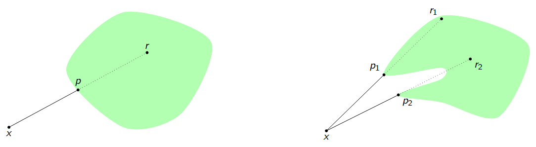
\[R_S(x) = 2P_S(x) - x\]Essentially, \(R_S(x)\) “reflects” \(x\) into the set \(S\), for visual intuition, see this illustration by Matthew Tam.
Assorted pedantry
Projection, and reflection is set valued. This is a fact I will consciously ignore over the rest of this article. Help participate in this doublethink with me, and if this topic ever confuses you, pretend that the projection operator also arbitrarily chooses an element from the set.
Additionally, the sets we’re dealing with will be closed and nonempty, so projection is always defined. Please scream at me if I forget to include these in theorems.
Example projection
While projecting on a set sounds like an even harder problem to solve than finding the intersection of sets, there are very many sets for which projection is known and easily calculated, like hyperplanes and hyperspheres. However, even for sets with a combinatorial flavour, projection can be surprisngly easy to compute.
Projecting onto the set of permutations
Consider the set \(S \subseteq \reals^n\) where \(c = (c_1, \dots, c_n) \in S\) iff \((c_1, \dots, c_n)\) is a permutation of the integers 1 to \(n\).
Claim
\(P_S(x) = (b_1,\dots, b_n)\) where \(b_i\) is the new index of \(x_i\) after sorting \((x_1, \dots, x_n)\) in ascending order.
Proof
We wish to find the \(c \in S\) that minimises \(\lVert x - c \rVert\), or equivalently we can minimise \(\lVert x - c \rVert^2\). Expanding, we get
\[\lVert x - c \rVert^2 = \lVert x \rVert^2 - 2 x \cdot c + \lVert c \rVert^2\]Observe that since \(c\) is a permutation, all \(c \in S\) have the same magnitude. Additionally \(x\) is constant in \(c\). Hence we wish to find the \(c\) that maximises \(x \cdot c\)
Now we use the rearrangement inequality- which tells us to maximise the value of \(x \cdot c\), we need to arrange the values of \(c\) so that the smallest value of \(c\) matches the smallest value of \(x\), the second smallest of \(c\) with second smallest of \(x\), and so on. This process results in the definition of \(P_S(x)\) as seen above.
Implication
\(P_S(x)\) can be calculated in \(O(nlogn)\) time. Wow.
In fact, many combinatorial sets tend to have the same idea of sorting, utilising a similar rearrangement inequality argument.
Cyclic projections
How do we use our projections to solve feasibility problems? A very natural first idea would be to initialise some \(x_0\) to some arbitrary point in \(E\), then iteratively project to set 1, then set 2… then set \(n\), and then cycle back around to set 1. Heuristically, it’s like we are trying to consider every single set in some systematic way.
This method has a long history and can be traced back to at least the work of von Neumann in 1950, where he proved convergence for \(n = 2\) subspaces. Today, we know that so long as the sets are convex, then the algorithm will converge to the intersection when it exists.
A more concise definition
Given \(n\) constraint sets \(C_1, \dots, C_n\), choose an arbitrary \(x_0 \in E\), then define the following sequence
\[x_{k+1} = (P_{C_n}P_{C_{n-1}} \dots P_{C_1})(x_k)\]When the \(n\) constraint sets are convex and the intersection is nonempty, then \(x_k\) converges to an \(x \in C_1 \cap C_2 \cap \dots \cap C_n\), no matter the starting point \(x_0\).
Douglas Rachford Algorithm
Another popular and well-studied algorithm is the Douglas-Rachford algorithm. This algorithm solves feasibility problems with 2 constraint sets, \(A,B \subseteq E\)
First, initialise \(x_0\) to some arbitrary point in \(E\). Then calculate the sequence using the following iteration step:
\[x_{k+1} = \frac{1}{2}x_k + \frac{1}{2}R_B R_A x_k\]What an odd iteration step! I honestly still do not have a good visual intuition, and this specific operator still feels extremely arbitrary. However, it is what it is, and here are the following properties.
When \(A\) and \(B\) are convex and \(A \cap B \neq \varnothing\), then \(P_A(x_k)\) will converge to a value \(x \in A \cap B\), no matter the starting point \(x_0\)
Comparing Douglas-Rachford to Cyclic Projections.
It’s almost a disappointing result- it seems as if Douglas-Rachford does what cyclic projections do, but constrained to 2 sets. However, as it turns out, there is an additional fact about its that can be proven about this algorithm.
Even when \(A\) and \(B\) are non-convex, if \(x_{k+1} = x_k\), then \(P_A(x_k) \in A \cap B\)
In non-convex settings, cyclic projections does not have this property, and often gets stuck in fixed points that aren’t the actual solution. This theorem tells us that Douglas-Rachford will not suffer from this problem. Of course, there are other ways Douglas-Rachford can fail to converge in non-convex settings. For example, it can get stuck in a cycle, or blow up to infinity. More concrete examples coming later in this article.
Running this algorithm on n > 2 sets anyways
We can even do some nice trickery to get this algorithm to work on \(n\) > 2 sets! Suppose we had \(n\) sets \(C_1, \dots, C_n\). Define new constraint sets \(\mathbf{C}, \mathbf{D} \subseteq E^n\) so that
\[\mathbf{C} = C_1 \times \dots \times C_n \text{ and } \mathbf{D} = \{(x,x,\dots,x) \mid x \in E\}\]Clearly, if \(\mathbf{x} \in \mathbf{C} \cap \mathbf{D}\), then \(\mathbf{x}\) will consist of \(N\) identical copies of an \(x \in E\), and will satisfy \(x \in C_i\) for all \(i\).
If we have \(n\) sets, then Douglas-Rachford can still solve the feasibility problem by running it on \(\mathbf{C}\) and \(\mathbf{D}\) as defined above.
For avoidance of doubt, from here on out, we shall notate \(\mathbf{x} = (x_1, x_2,\dots, x_r)\)
Projections
Note that projections onto \(\mathbf{C}\) and \(\mathbf{D}\) can be quite easily calculated, we have
\[P_{\mathbf{C}}(\mathbf{x}) = P_{C_1}(x_1) \times \dots \times P_{C_n}(x_n)\] \[P_{\mathbf{D}}(\mathbf{x}) = (\frac{1}{n}\sum_{i=1}^n x_i, \dots, \frac{1}{n}\sum_{i=1}^n x_i)\]Malitsky-Tam Algorithm
My supervisor co-authored a paper proving a theoretical bound for the a certain class of algorithms- in the process constructing an algorithm that can be specialised to solving feasibility problems. However, its numerical performance isn’t well studied, and he personally wanted to know how it would fare against combinatorial problems- and that’s partly why I embarked on this project in particular.
A forewarning: We will now overload the power operator, and begin using superscripts as merely labels for vectors. Do not take \(x^k\) to mean “ \(x\) to the power of \(k\) “, but merely “ \(x\)-\(k\) “.
Given \(n\) closed sets \(C_1 \times \dots \times C_n \subseteq E\), initialise \(\bz^0=(z^0_1,\dots,z^0_{n-1})\in E^{n-1}\) and \(\gamma\in(0,1)\)
Then compute \(\bz^{k+1}=(z_1^{k+1},\dots,z_{n-1}^{k+1})\in E^{n-1}\) according to
\[\bz^{k+1} = T_A(\bz^k) = \bz^k + \gamma \begin{pmatrix} x_2^k-x_1^k \\ x_3^k-x_2^k \\ \vdots \\ x_{n}^k-x_{n-1}^k \end{pmatrix}\]where \(\bx^k=(x_1^k,\dots,x_n^k)\in E^n\) is given by
\[\begin{cases} x_1^k=P_{C_1}(z_1^k), \\ x_i^k=P_{C_i}(z_i^k-z_{i-1}^k+x_{i-1}^k) \qquad \forall i\in \integ{2}{n-1} \\ x_n^k=P_{C_n}(x_1^k+x_{n-1}^k-z_{n-1}^k). \\ \end{cases}\]where the notation \(\integ{a}{b}\) denotes “The set of integers between \(a\) and \(b\) inclusive.”
Convergence
If the sets are convex, then \((\bz^k)\) converges weakly to a point \(\bz\in\Fix T_A\) and \((\bx^k)\) converges weakly to a point \((x,\dots,x)\in E^n\) with \(x\in\bigcap_{i=1}^nC_i\).
That’s it!
That’s all the mathematical preliminaries, thanks for hanging in there. In the next part, we will explore our first feasibility problem, nm queens
I’ll show you how to formalise the problem as a feasibility problem, how the two algorithms performed, and how I poked and prodded them to learn more about how they work.